Future City: Update 11 - Block Interfacing

Progress on Future City has been slowed by web-site and release preparation work at the moment.  I've split my time about 2:2:1 between Web site, Future City, and Alpha Release preparations.

January push towards Web Site, City demo, and Alpha Release.

This split in attention as well as the pressure of the approaching alpha release means blog posts have been slower forming.  Let's just squeeze out a quick update on the Future City progress...

Future City

At the moment I've been focusing on the support of variable elevation across the city, with each city block having its own height.

Example of blocks with shared connectivity but height discontinuities

This feature results in rather complicated requirements at the interfaces between blocks as well as complicating the process of sub-dividing up the space within them.  As such, it's been quite slow progress working out (a) exactly what is required, (b) how to perform this, and (c) how to implement this.

Requirements

Based on the previous connectivity work which sub-divided the city up into districts/zones and finally blocks, we have already decided on what the connectivity between each block looks like.

Now we need to decide on what the content of the block should be such that it is possible to guarantee that adjacent, separately generated content aligns properly, functions as a seamless transition, and looks plausible.

Inputs

We have the following information about each block boundary:

• Block location/bounds/size.
• Access along each side (left/right of opening within any barrier present).
• Follow the underlying landscape shape, or both share flat ground level at a given height.
• Connectivity via each side (to the outer most city sides).
• Variation seed to drive arbitrary design decisions.

Outputs

From this we need to populate the block with rectangular sub regions.  The main problem we are trying to solve here is to transition from a boundary with zero, one, or two accessibility transitions along each side into spaces for content to go that all have single accessibility along each side, these being simpler requirements to satisfy.  Thus the outputs are of the form of Content Spaces with the following properties:

• Bounds size, orientation and location
• Surface height within the space (or if we are to follow the landscape)
• Is it an interfacing piece, i.e. responsible for handling transition to neighbouring block interface? (Edge - one interface along block boundary, Corner - two interfaces along block boundary, Side - three interfaces along block boundary)
• If not an interface, then an interior piece, with same type all round (flat or landscape)
• For each boundary interface: Specific flat elevation or landscape following. Do we 'own' this side (are responsible for interfacing geometry). Is this a barrier, i.e. will access be blocked? Is there a barrier to the left/right that we may need to provide transition geometry for?

Test Rig

Since there are a lot of combinations to test in forming this system it is worth generating a set of 'unit tests' with clear visualisation of the inputs and outputs.  By creating a hierarchy of test procedures we can quickly generate tests for all the major side and access combinations.

• Ownership - all, none, adjacent, opposite
• Surfaces - all landscape, all flat, mixture
• Access - Closed corners, all open, all closed (bar one), some on left, some narrow, mixture

Unit tests for a lot of the block interfacing cases

For cases where a specific issue is being resolved there is the option to switch out all but one test scenario.

Example test rig showing corner results produced

Algorithms

I spent a lot of time in Excel playing with block boundary examples and possible approaches.

Playing with block algorithm ideas in Excel

From this I've come up with a lot of ideas, but they seem to be heading towards this sequence of calculations:

First pass at the content space and interfacing algorithm

There are bound to be some changes as implementation proceeds, but this is a good starting point.

Lists

Structured Data

The amount of structured information and variability in generated output finally became too much and I had to stop to add some functionality to help support this.  Previously where several properties about a single thing needed to be conveyed through several procedures it had to be passed individually, and explicitly.  This leads to this specific flavour of spaghetti:

A specific flavour of spaghetti: arrays of connections

The algorithms that were forming to perform the interfacing and content-space generation were heading towards an awful lot of this.  From the requirement analysis above we can see each block has at least seven properties that go together, and each potential output content space has at least six.

Traditionally these would be encapsulated in structures, where a single type is used to express an explicit collection of typed data.  This is something that Apparance will natively support in the future, but it's quite a lot of work, especially on the tooling side where composition/decomposition of structures needs to be handled elegantly.

Variable Quantities

Another aspect of the block interfacing implementation problem is that there are several places where we need to pass a variable number of structures.  At the moment there is no concept of this and we would have to pass a fixed (maximum) number of structures (as individual properties) along with an additional flag expressing whether it was in use.  This forms a very, very unwieldy situation where all sorts of operations, such as combining two variable sized collections, become incredibly complicated, expensive and error prone.  We really need some form of list or array to handle this.

Solution

Both these prospects are really going to cause too much of a headache to work on the already complex problem, so we need support to help this.

Looking at other language for inspiration, we find that both these problems can be addressed by using lists of dynamically typed objects.  If a list happens to contain all the same type, then it is effectively a traditional list or array, i.e. a variable sized collection.  If a list happens to contain a fixed number, of different typed elements then it can be used as a structure.  Adding support for lists as just another base data-type to Apparance is fairly straight-forward and then means we can have lists of lists, or put another way, lists of structures.

Implementation

The List data type was added along with an initial set of basic operators to support what we would need, as follows:

• Append - take a list and add another element (any type).
• Get - index a list, returning the element value (any type).
• Set - replace a value at a specific index with a new value (any type).
• Count - query how many elements are in the list.

Part of the implementation that took a bit of effort was that I wanted type information to be maintained with them as the lists are constructed.  With this, a lot of validation can be performed during synthesis that would catch problems that would otherwise be very difficult to diagnose and have potential to crash the engine.

Whilst a bit tricky to implement, lists are proving very useful so far and make a lot of the block interfacing problem much more pleasant to work with.

Passing structures and collections around as lists

I am even now using them in the web site building procedures for all sorts of things.

Progress

I'm about half way through the Block Boundary -to- Content Space processing system and have promising results so far.

Some of the content space generation results so far

I'll post more results as I progress.  In the mean-time I have an Alpha Release to get out!

Future City: Update 1 - Divide And Conquer

Top Down

A key consequence of the Apparance detail management system is that each stage of refinement must be possible independently from any other.  The upshot of this is that the content within a block (in a particular tier) must only depend on the content of its parent (higher tier) block.  It can't depend on the content of any neighbouring blocks.  If this were allowed, then you introduce many cases where long chain dependencies and circular dependencies occur causing no end of problems.  It is also easy to see that approaching a block from one direction leads to neighbouring blocks being refined in a different order to approaching from another direction, again causing problems if you depend on them.

Vertical (downwards) dependency = Good :)
Horizontal (sibling) dependency = Bad :(
Circular dependency = Really Bad :( :(

The Price We Pay

For a lot of structures and models we may want to build, this constraint isn't a problem. For example, refining a wall into individual bricks is straightforward as the bricks and their positions can be generated deterministically from the more general wall shape representation above.  There are however many cases where we cannot model in this way, for example; building a dungeon of interconnected rooms and corridors.  Many procedural dungeon generators are effectively image processing systems, applying several passes to the dungeon 'image' (cells or otherwise) to build up, interconnect, and validate the space.  This is illustrated well in this nice dungeon generation write-up.  Since Apparance doesn't have any image processing (yet) with which to drive this sort of generation, and is effectively a purely functional programming system, we have to use the sub-division approach and work out how to circumvent the horizontal inter-dependencies we meet when neighbouring rooms need to be connected.  More on this later/next time.

City Size

As an initial starting point I think a 10 km x 10 km* city is a good mixture of being both an impressive size and suitable technology show-case.  Since we are always sub-dividing, we also need to start with an outer frame for the city that is big enough to house the tallest building we want.  To put this another way; setting the starting height of the city frame defines what the maximum height a building can be.  (It's a mindset that we need to really get into to).  A height of 200 m* is a good starting point; here's what it looks like:

Bounds of our 10 km x 10 km x 200 m city

*The engine is generally unit agnostic but I am going to stick to 1 Unit = 1 m for sanity's sake.

Space Filling

As stated previously, we are limited to rectangular sub-division of the city at the moment so it will all be a bit angular, but hopefully arbitrary splitting and plenty of adjacent zones with the same type will create interesting shapes none-the-less.

An algorithm I've used before to divide up a rectangular area is as follows:

1. If too small to subdivide, instance a zone and return.
2. If we aren't forced to subdivide (because we are too big), optionally instance a zone and return.
3. If we are too small in one direction then subdivide in the other direction, otherwise choose a direction.
4. Choose a split point such that no sub-regions are too small to instance.
5. Split into two parts and recurse into each part in turn.

This works well and was basically what was used in some early dungeon generation experiments.

Here is this algorithm implemented as a procedure in the Apparance Editor:

Recursive city zone subdivision procedure

This one is mostly fundamental operators (grey block), but the three white blocks are procedures; 'Content' is where we instance a zone, and the 'Zones' procedures are instances of the procedure itself and where the recursion happens.  There are two, one for each side of the split point.  It's a fairly complex procedure as they go, so if you have specific questions about it let me know in the comments below.  The longer lines crossing over behind other operators make it a bit messy but I have ideas about how this UI could be improved (another story).

Setting up the content procedure to just render a randomly coloured inside-out box and choosing suitable minimum and maximum zone sizes gives us a nice visualisation of the resulting zone layout.

City zone procedure output. Zone sizes from 500m to 2,500m.

City Structure

To model an interesting city layout I decided that some familiar planning approaches should be used.  We will start with some basic city district types and a mechanism for loosely specifying where they should be located in the overall city.  This can then be used to drive the classification of each zone as we divide up the city.

• 1 business zone (offices, skyscrapers)
• 1 commercial zone (shops, restaurants, tourist attractions)
• 1 industrial zone (chimneys, factories, and storage facilities)
• 1 space port zone (space ship docking and handling)
• Leisure zones (parks, monuments, and recreation areas)
• Residential zones (housing)

The last two are to be used to in-fill the remainder of the map and don't have any specific location.

Zones are going to form the highest level of city structure, and eventually each one will have many buildings and areas within it (probably called 'blocks', like city blocks).  For now, we are laying out the general plan.

Zone Distribution

For each instanced zone, we need to weigh up the various factors that affect what it could be:

1. Distance from each district centre.
2. Size of each district.
3. Weightings of the non-centralised district types.
4. A random factor to introduce variation and avoid clean district boundaries.

This is embodied in the following procedure:

Main zone type calculation procedure

Here, we use the zones location (centre point) to calculate weightings for the four centralised districts and then perform a weighted selection between them to generate a zone type (an index, 0 to 5).  We'll dig into each of these in turn:

Design Parameters

I've found it useful to group design-time constants into their own procedures.  These are effectively global variables, but with the option of making them parameterised later too.  Doing this makes it easy to find major control points by just looking for procedures named 'Design' in the procedure browser when it comes to tweaking the project later on.

Zone design parameters wrapped in their own procedure

Here we have grouped the zone min/max sizing values as well as all the location, size, and weighting parameters used in zone type selection.  For convenience, I have encoded the district size in the Z value of the Vector3 as only the X and Y are needed to specify a centre.  (Structure support is on the wish-list, but a long way off).

Zone Weighting

This is a fairly simple procedure that just takes a zone location and a district definition (labelled Zone Centre & Size here) and generates a weighting value.  The convention here is that you get a weight of 1 at the centre and a weight of zero at a distance of 'Size' from the centre.  This will generate negative values outside of that but this doesn't affect the weighted selection process.

Zone weighting calculation

Distribution

The distribution process is a general one and hence the procedure was created under the 'Maths' category (for want of a better location).  This is implemented as a chain of tests to see if each weighting value should replace the previous one.

Distribution evaluation via chained tests

Several outputs feed into the next test in the chain, with the final result being available at the output of the last test.

Individual distribution test procedure

The test procedure performs a weight adjustment according to the dithering parameter, randomly offsetting the weight a little to introduce artificial successes and failures when comparing against similar weights.  This introduces an amount of overlap between the district types.  The weight is compared with the previous 'best' weight and this selects whether its own index and weight are passed on, or the previous stages index and weight.

The Results

Updating the Content procedure to colourise the zone according to district type and putting all the above procedures into action produces the following, rather satisfying, result:

City zones classified into district types

Here you can clearly see four of the colours (red, yellow, green, and cyan) are centred around specific points in the map and the other two (blue and magenta) are mixed in around them.  The dithering has been adjusted to break up the zone boundaries and we can see some impinging of the residential and leisure district types on the centralised ones.

As the procedures were constructed, any element of random choice is driven from seed values passed down through each procedure.  This means that the seed value passed into the root procedure can be changed to affect the whole city.  Here are a series of district layouts from a series of seed values:

Varying the seed to produce different cities with similar structure

Each one still has the general layout desired, but introduces interesting variations on the same theme.  Later on we can experiment with parameterising the design parameters so that the locations, sizes, and weightings of the districts themselves can change from city to city.

Next

The next step is to look at how these zones are going to be connected, what sort of interfaces there will be (free travel, steps, ramps, barriers, etc.), and how we are going to break these blocks up further and start to introduce actual buildings.

The Procedure Authoring Process

Being a visual tool where all content is created within the editor it is of paramount importance that the authoring process is a smooth one.  The tools and UI are being developed to be a low friction and intuitive experience, and I am always thinking about ways to improve them.  Let's take a look at the procedure authoring process.

Managing Procedures

The first step is to add a new procedure to the procedure browser.  Pressing Alt+N creates one called "new procedure".  It will inherit the category of the currently selected procedure.  Single click to select a procedure (highlighted in yellow) and you will see its properties appear in the property panel.  Here you can change its name from the default to something suitable.  If you want, you can change its category too.  As you rename or re-categorise a procedure it will move to the appropriate place in the procedure browser.  Scroll around or use the filter box at the top of the panel to find it.

Creating a new procedure

Procedure Files

A procedure is stored as XML data in a .proc file on disk, along-side this lives a .procedit file containing any data that is only needed in the editor such as visual graph layout and element descriptions.

Procedure files and their editor data companions

Each category has its own folder on disk.  As you rename/recategorise a procedure, these files are renamed and moved around accordingly.

Viewing & Editing

When you are working on a procedure you will probably want to see the results in the 3D view, to make a procedure the subject of this view select it and press the View button at the top of the browser panel.

To edit the procedure content, either select it and click the Edit button or just double-click on it and it will open in the procedure graph which we will look at next.

Editing and Viewing a new procedure

Procedure graph

The main part of the editing window is dedicated to viewing and editing the procedure graph.  A procedure has a perimeter surrounding it's content as well as hosting the input and output connections for it.  The procedures title appears at the top of this area, inputs on the left, and outputs on the right.

The viewing area can be panned around by holding the right mouse button and dragging, and zoomed in and out using the mouse wheel.  Normally the view is fully zoomed in and you will only need to zoom as you work on larger procedures.

Operator Instances

The most important part of creating a procedure is the adding of operator instances into it.  This is done by dragging an operator from the procedure or operator browser panel onto the procedure.

Placing operators by dragging onto procedure

New instances are unconnected and have default values for all of their inputs.  Operators can be removed by selecting them and pressing Delete.

Selection & Manipulation

Operators (and procedures) placed in your procedure can be singly or multiply selected to allow movement, and input value editing.  Shift+Click to add to the selection, and Control+Click to toggle inclusion.  You can also drag a marquee (from an empty part of the window) around operators to select them.  Click on the empty background to deselect.

Selected procedures can be dragged around to be repositioned, both individually and in multiselected groups.  If you move operators near to the edge of the procedure the boundary will be expanded to accommodate it.

Wiring

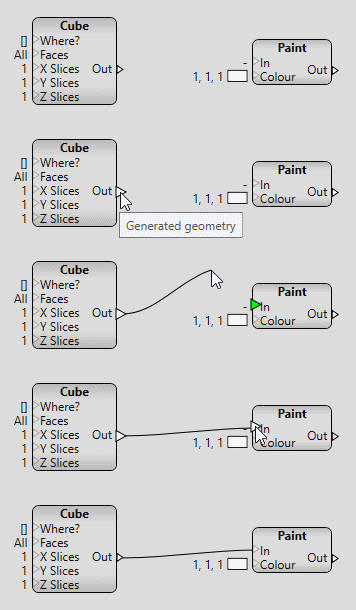
To use an operator it needs to be connected up with the visual wiring metaphor we use to show where inputs should get their values from.  Each input and output has a name label and a connection point.  Hovering over a connection point and dragging creates a wire attached to that point.  You can now interactively choose the appropriate connection point you want to connect to.  Compatible connection points (same type) are highlighted during this process.  Hover over the target connection point and release the mouse button to make the connection.

Connecting operators together

Existing wires can be moved around easily by grabbing one end and dragging it to somewhere else.  As you hover over a wire it will highlight, both the whole wire (thicker) and one of the ends (white).  This helps you see what a wire is used for in a complex procedure, as well as allowing you to specify an end to be reconnected.  If you drag a wire and drop it away from any connection points the wire will be removed.  Any disconnected inputs will revert to their previously set constant value.

Highlighting and disconnecting wires

Constants

Operator instances with unconnected inputs assume a constant value.  To specify this value simply select the operator and the property panel will list its inputs and values for editing.

Editing an operator instances input values

Connected inputs can't have their value set as they implicitly get their value from another output which is evaluated at synthesis time.

Procedure IO

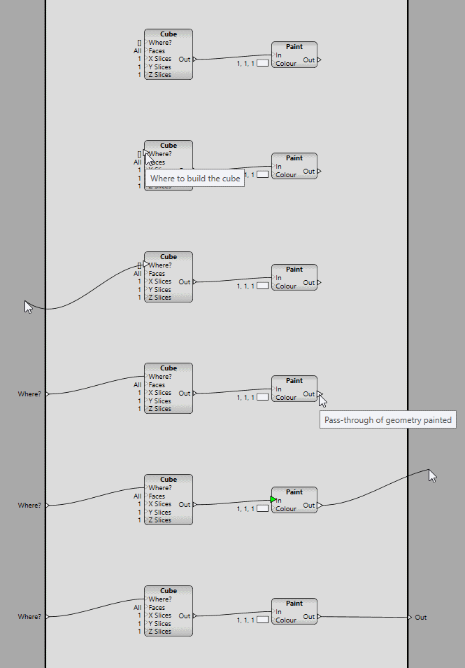
Procedure inputs (along the left edge) and outputs (along the right edge) are created by starting a new wire on an operator output or input and dragging it outside the procedure boundary.

Creating procedure inputs and outputs

By default this new input/output assumes the name and type of the operator connection point you start from but they can be edited in the property panel by selecting the whole input or output area.

Editing procedure inputs

Editing procedure outputs

Procedure inputs and outputs can also be selected individually for editing, or removal (press Delete).

Once created, procedure inputs and outputs remain present and can be connected/disconnected/reconnected the same way as operator instance inputs and outputs.  In fact; procedure outputs behave exactly like operator instance inputs and procedure inputs behave exactly like operator instance outputs.

Notes

To help document procedures, visual notes can be added.  These are rectangular panels with a title and description text you can adorn a procedure with to explain what is going on.  You can also use them to surround operators to group them such that they can be moved around as a unit.  To include/exclude an operator from a group just drag it into or out of the note boundary.

3D view

The currently viewed procedure is submitted for synthesis and the resulting models displayed in the 3D renderer view-port.

The output of our procedure shown in the 3D view

As edits are made to the procedure structure and constants it is regularly re-submitted so that the models update to reflect these changes providing interactive feedback for your design.

Interactive editing of procedure data

Camera

The 3D view provides a standard range of camera controls including:

• FPS style navigation - right mouse button to look around, WASD to move forward/strafe plus QE to raise/lower.
• Modelling camera - Middle mouse button to pan, with Alt to orbit, with Control to raise/lower (Z axis), with Shift to move around the XY plane.  The mouse wheel can be used to adjust the orbit distance.
• Auto-rotate - left click to toggle a carousel style orbit mode.

Grid

By default, the 3D scene includes a ground-plane grid and an axis indicator at the origin to help visualise the 3D space and scale of objects modelled.  This can be disabled and adjusted if needed by clicking the Grid tab at the top.

Drawing aids and their settings

Expanded View

The normal 3D view is fairly small but fine for a lot of modelling needs.  For cases where more detail is needed though you can toggle it to large size by pressing the Space bar.  In this view you only have the 3D view and the property panel visible.  This is a great mode to tweak values in.

Toggling expanded 3D view

Property Editing

Many elements in the editor can, when selected, have their properties displayed in the property panel for review and editing.  This used for operator input constants, procedure properties, synthesis and rendering statistics, and grid and view-port diagnostics settings.

Types 

Most data types are view-able and editable in the property panel, including; integer, floating point, boolean, colour, string, vector, and even frames have basic editing control.

Controls 

Some types have specialised controls, for example, numerical values have a slider control to aid interactive adjustment.  The minimum and maximum range of the slider is editable too, and stored with the procedure so it is there for convenient editing of the value next time the procedure is opened.
Integer inputs can also be set up in the operator definition to have enumerated values.  This can be presented as a drop-down selection or a series of buttons.  Inputs that represent a set of flags can have independant toggle buttons for each flag as well as some composite value buttons, e.g. All, for convenience.

General

A few of the more general features of the editor are worth mentioning.

Undo

Most editing operations, including property changes are command based and enable full undo/redo support.  The usual Ctrl+Z/Ctrl+Shift+Z keys are used to navigate the command history. 

Save & Load 

Procedures with unsaved changes show in bold font in the procedure browser.

Unsaved procedures appear in bold

Pressing Ctrl+S or the Save button at the top of the browser will save all unsaved work in one go.  The save process is two stage and uses temporary intermediate files to protect your data from problems during the save process.  All procedure and editing files are also kept in a back-up history.  This is stored in a backup folder alongside the procedure files.

All procedures are loaded at startup by default.  This makes managing them much simpler.

Updates

It's worth mentioning how procedure updates are propagated and applied to the models in the 3D view.  Any time you perform an editing operation on a procedure, it can potentially affect the generated output.  By following the dependency graph back from the edited procedure a list of all potentially affected procedures can be built.  This is then used to determine if the procedure you are viewing needs to be re-synthesised.

If you are adjusting a slider and potentially generating lots of edits in a short space of time the engine will try to update as fast as it can without swamping the synthesisers.

Summary

The functionality described here corresponds to the current state of play.  This is the tool set I am currently using to build and test procedures.  There is lots of scope for improvement and I have a large wish-list of features and tweaks to add.  Usually these are implemented when I am building more involved demonstration procedures and find bottlenecks in the process.

Next

I am going to be away for a couple of weeks so the next few blog updates may not be as regular as they have been so far.

A Look Around The Editor

For this post I'll show you round the different parts of the editor application's user interface.  Next time I'll dig into the editing functionality and how to use Apparance to actually build procedures.

An Editor?

Why do we need an editor?  Well, we are trying something very different here, by way of workflow, modelling paradigm, and output.  As essential parts of the Apparance concept, building a custom editing application was the only way to achieve this level of bespoke requirements.  Some of the important features it needs are:

• Creation and management of procedures
• Data-flow based visual graph editing
• Preview of resulting procedure output
• Real-time, interactive authoring and tweaking

Looking through the image gallery you can see how the user interface developed.  Initially as I was proving the procedure data representation and the synthesis process it was just driven as raw XML data.  This was fine for testing, but as you can imagine it was incredibly unwieldy for anything but very simple procedures.  As the project progressed I worked on each of the main interface elements in turn, improving them again and again.  Let's look at them in more detail.

The Apparance Editor

Browser

Good design means factoring out functionality into smaller, re-usable, chunks, and consequently we will need to be able to work with many procedures.  At the moment, procedures are organised in a simple two level hierarchy with a Category and a Name.  This will probably need expanding in the future, for larger projects, but provides a way of grouping procedures together for now.

Procedure/Operator browser and properties of selected procedure

A browsing panel lists all the procedures and as a navigation aid there is a filter box to narrow down those displayed.  As well as procedures, the fundamental operators they are built from are also listed, in their own browsing panel and can be filtered in the same way.

Procedure Editing

Once you create a procedure you need to start specifying the functionality within it and the connections in and out.  This is performed within the main area of the editor in a scrollable, zoom-able window.

Zoomed-out overview of a large procedure in the editing window

Often your operator graph will fit within the window, but for more complicated creations you will need to zoom out or pan around.  Operators are boxes with the name of the operation at the top, inputs on the left, and outputs on the right.  The procedure itself has its inputs on the left and outputs on the right too.  Consequently, the natural visual 'flow of data' is from left to right, most connections and chains of functionality propagating information to the right.  This doesn't mean you can't make connections in any direction and create all manner of spaghetti. Careful factoring out of messy bits into sub-procedures helps here.

The inputs and outputs of the procedure that you specify and name here are what you will see and be able to connect to when you place your procedure down within another procedure.

Procedure IO editing

3D View

There is a rendering window in the corner of the editor where you can view a procedures output.  At the moment all output is 3D model geometry, and as we are targeting 3D worlds this is all you need to see a model in place.

The 3D preview window

By electing to view a procedure, you are specifying the starting point of the geometry synthesis process.  In order to do this with procedures that have inputs, you need to be able to specify their values.  This can be done where you edit the input connections to your procedure (see above) and are effectively the default values your procedure comes with.  This means you can preview any procedure as each come with some starting values.  These are also the values your procedure starts with at its inputs when you place it down.

The 3D view-port has pretty standard camera navigation controls, with orbit, and FPS style movement as well as an auto-rotate mode for showing off a model.

To help with construction and spatial orientation, a ground-plane grid is drawn for you.  This is implemented as another procedure that can be edited just like any other if it needs customising (e.g. turn off, adjust colour/intensity, spacing, scale, etc).

To get a better look at your scene you can expand the 3D view to occupy the whole editing and browser area.  This leaves the property editing panel (which expands to occupy the space where the 3D view was).  This mode is ideal for tweaking values, simply select the operators who's inputs you want to change and switch to expanded mode.

Toggling the large 3D preview window

Property Panel

Most editing environments include some form of properly panel where a list of the individual adjustable elements of an object are shown.  The Apparance editor uses this for editing (and viewing) a number of things, such as: Operator input constant values, procedure IO name and description, new procedure name and description, renderer settings and statistics, view-port visualisation modes (see below) and diagnostics, and grid settings.

Property viewing and editing panel

Most data types are fully editable, some with specific enhancements such as sliders for floating point values and toggle buttons for enumerations.  Sliders have editable min/max values too so you can set them to a sensible range for the value the slider controls.

Development

In line with the live/interactive editing model adopted here, most of the user interface can be updated at run-time.  This has made development of the UI much, much faster and allowed much in the way of polish that would have otherwise been left.  The editor UI is implemented in WPF which supports dynamic loading/parsing of the backing XAML design data.  Custom text editing panels can be expanded to allow live editing of most of the editor interface.

Live editing of the editor UI

The synthesis process can be monitored in a custom panel showing each of the synthesisers, with a timeline of the jobs each works on.  For each job a breakdown of memory use and any issues encountered is displayed.  This is needed to diagnose any technical modelling problems.

Synthesis statistics and diagnostics

Another panel allows exploring of the internal engine structure and any properties exposed by each part.

Engine exploration; here showing view-port modes and settings

There are a few ways to analyse the operation of the engine, the synthesiser, the procedures, and the tools, including: GraphViz dumps of each synthesis run, the scenehierarchy, and procedure capture analysis process, as well as in-editor visualisations of the detail refinement hierarchy, the editor tool stack, and the UI stack.  All helpful in working out why things aren't going as expected and important to understand how best to build procedures that work well with the engine.

Next

Next time I will talk about procedure creation, editing, and viewing.

An Introduction to Procedures

As there is a huge amount to cover I'm going to spread it out over multiple posts.  The first few will describe the technology (engine) and after that I'll cover the tooling (editor).  This will by no means cover all the technical detail, but it should give you a good idea of how it works and what (I hope) it will be able to do.

Authoring

Currently the engine allows building of procedural models; objects formed of triangles (and lines) and rendered in a 3D viewport.  These are expressed as 'procedures'; collections of modelling and calculation operations that feed into each other forming a network or graph.  The 'inputs' to this are various constant values within the graph and the output is a 'value' corresponding to the generated geometry.

A simple procedure and the resulting model

Each node is some form of fundamental operator (like add or subtract) implemented in code, or it can be another procedure, itself made from operators and procedures.  The term 'operator' will be used to mean either in the context of a procedures content as once placed down they can be treated in exactly the same way.

A multiplication operator feeding into a luminance procedure

Each operator generally has one or more inputs and one or more outputs, which can be connected up to other operators.  An input can only be connected to one output but an output can connect to multiple inputs.  There are several fundamental data types available for information to be passed between operators.  So far we have: Integer, Float, Bool, Colour, Vector, Matrix, String, Frame, and Model Segment.  These last two are explained more below.  Unconnected inputs are considered constants and the value can be explicitly specified.

Operator inputs of various data types

When creating a procedure, you get to define it's inputs and outputs, and their names and types, these then become available for connecting-to wherever an instance of the procedure is placed down.

Procedures represent blocks of functionality and can easily be used to encapsulate and re-use groups of operators.  For example you might build a colour blend procedure out of mathematical operators if a dedicated operator wasn't available or didn't meet your needs.

Bespoke colour blending procedure

The new blend procedure in use

Operators

There is a small library of built-in operators implemented already to build procedures from, these are roughly divided into:

• Mathematical operations - all the usual maths functions.
• Comparisons and conditional switching - test and flow control.
• Conversion - e.g. changing type or break-out/re-combine (for multi-element types).
• Constants - operator inputs are editable constants, but constant operators are useful for sharing values.
• Modelling - create and manipulate primitives (cube, cylinder, paint, distort, etc).
• Space defining - subdividing and specifying spaces to be used for containing objects (Frames).

Some of the operators available so far

There are hundreds more of these I need to support (something for a future post), but this is plenty for me to test and prove out the principals.  In fact this current limitation means I have to be inventive and really means I push the capabilities of the procedure system to see what I can achieve.

Modelling

Currently there are only two triangle primitives (Cube and Cylinder) and two line primitives (Line and Grid).  The only reason I haven't written more yet is that I have managed to achieve a surprising amount with just these.  All the screenshots you can see so-far are mostly built with the cube operator and an occasional cylinder.  As we will see though they do provide a fair bit of control over how each can actually be used.

Once I got to the point where the geometry synthesis was basically working and I started building shapes I found that a large part of building up objects is actually splitting up the space it is going to occupy into smaller spaces.  This happens at many depths and in many different ways.  There are parallels here to laying out elements on a page or in a user interface, so many concepts like centring, distribution, and offsetting apply equally to 3D space. To facilitate this in Apparance I found a data type to describe an oriented cuboid in space was ideal for this.  These I call 'frames' and operations on them form a large part of the object construction process.

Space partitioning operators in use (highlighted yellow)

Starting with a frame describing the location, orientation, and dimensions of the object being created, you break it down into sub-frames until you reach a point where a single primitive fits exactly, at which point you feed the frame into it generating the geometry needed there.  This aspect of modelling needs a post to its self really :)

Geometry generated by a primitive operator is passed around the graph using a 'Model Segment' data type.  This rather esoteric type is just a way of remembering where in the modelling buffers the vertex and triangle information for that primitive has been put.  A 'combine' operator is available to merge two segments of geometry together so they can be treated as one.  All modelling should result in a single Model Segment output at the top level and it is the geometry enclosed within it that will be displayed.

Part of the appeal (to me at least) of procedural generation is parameterisation.  Anything we build this way can have any aspect of its form exposed as a tweakable parameter.  This may just be the desired size of the object, it might be the thickness of the frame on window, the colour of a building's roof tiles, or the probability of a wonky brick in a wall.  In order for a given parameter to affect the modelling process its value will usually need to be massaged into some other form by using mathematical, conditional, and logic operators.

Synthesis

The process of turning procedures into models that can be rendered it called 'synthesis'.  Starting with a root procedure to be viewed in a 3D scene the synthesis engine starts by instantiating it in memory with any input values needed and requests the geometry via the appropriate output.  This triggers instantiation of all the operators within and their interconnections.  Following the 'flow' of the data connections back from the required output and digging down into procedure within procedure all the functionality needed to produce it is executed.  Requests for output values from leaf operators, ones with actual code behind them causes that code to be executed.  Procedures and operators also call upon their inputs which then cause the evaluation to elevate back up to the level above and follow the connections already in place when the containing procedure was evaluated.

Evaluation tree for the table example

Because procedures are instantiated as they are needed, it can support recursion, i.e. a procedure can include instances of itself.  As long as there are 'exit conditions' defined to limit the recursion depth this turns out to be a really useful way to build a lot of structures.  I discovered early on that this can be used to implement arrays of objects by progressively subdividing until the required object size was reached.  I thought I would need array support explicitly but so far recursion has served well in its absence.

A recursive procedure called "Recursive" that includes itself.

Output of the recursion example

To help with scalability and performance, multiple synthesis runs can be performed in parallel on several separate synthesiser instances.

Four synthesisers running in parallel, busy building geometry

Each has its own pre-allocated chunk of memory as working buffer, used in a non-freeing manner and only reset at the end of each run.  This makes allocation of parameters, values, operator state, and any intermediate data extremely fast and all values effectively immutable, simplifying the operator graph evaluation logic.

A breakdown of how memory was allocated during synthesis

Next

Quite a lot to absorb I'm sure.  I'm happy to answer any questions.  Next time I'll talk about the renderer, some of the less glamorous code supporting everything, and how the project is set up.